Measuring Microbial Growth Rates in a Plate Reader

The following protocol can be used to determine the growth rate of a bacterial culture using a plate reader by measuring the optical density (OD600) of the culture over time.

Program set-up

The parameters the Barrick Lab uses are:

• Temperature: Appropriate for growth of your organism
• Kinetic Cycle:

Duration: 16-24 hours (as appropriate for your experiment)

Kinetic interval: every 10 minutes

Orbital Shaking: 420 seconds at amplitude 3

Wait: 5 seconds

Absorbance reading: 600 nm, 25 flashes, 50 ms settle time

It's important for the program to shake for most of the time that you are not making measurements. Less shaking leads to slower growth.

Reviving cultures (2 days before experiment)

1) Grow an overnight culture of each strain being tested. Inoculate 2 μl of frozen glycerol stocks of each strain into 5 ml of media. Prepare a separate tube of uninoculated media as a control for contamination. Incubate overnight.

Preconditioning cultures (1 day before experiment)

Preconditioning acclimates the strains to the media. Additionally, on this day you should pre-warm your media as it takes a long time for the plate reader to warm up media. Not doing this will lead to inconsistent lag time.

2) Inoculate 5 μl of each overnight culture into fresh media to precondition. Prepare a separate tube of uninoculated media as a control for contamination. Incubate overnight. 3) Place the media you will use for the assay in an incubator at the correct growth temperature overnight to pre-warm.

Growing cells in plate reader and measuring OD600

All strains tested should have at least have 3 replicates, although more replicates should be performed as long as there is available space on the plate. Evaporation can occur in the outermost wells, so if there are few enough samples the outer ring of wells should be skipped. Due to small variations in temperature throughout a 96-well plate, best results will be obtained if replicates are distributed randomly across the plate. Clear Costar 96-well plates are a good brand to use.

4) Add 195 μl of pre-warmed media to each well being used for cultures and additional wells for blanks. 5) Inoculate each test well with 5 μl of overnight culture. 6) Place the plate into the plate reader. The lid can be removed (we've had no contamination, as seen on wells with LB blanks, or problems with this) 7) Start your program. 8) Once the program has finished, export the data as an Excel spreadsheet.

Fitting growth curves with Growthcurver

Growthcurver analyzes the optical density data by fitting it to a logistic function from which the growth rate, doubling time, and carrying capacity can be calculated.

Section in progress

References

1. Growthcurver publication: https://link.springer.com/article/10.1186/s12859-016-1016-7
2. Growthcurver manual: https://cran.r-project.org/web/packages/growthcurver/vignettes/Growthcurver-vignette.html

Contributors

• Isaac Gifford
• Julie Perreau
• Gabriel Suárez

Appendix

The following are instructions for calculating growth rates using Grofit, an R package that is no longer supported by the current version of R.

Converting your file with OD data to the proper format

What is most critical is the format and file type of the input data file containing the OD600 values. Most plate readers produce an Excel worksheet with the data results. With such a file, the first thing that must be done is to convert it to a comma delimited file. This is simply done by using "save as" in Excel and selecting *.csv as the file format. Your file should look similar to the one provided as example here:

• yourdatafile.csv: Example spreadsheet of your OD600 data file

Create a "times only" csv file

Grofit needs an additional file that will only have the times (e.g., 10, 20, 30 mins ...) for every time point measurement. An example of this file is given here:

• timesonlyworksheet.csv: Times only worksheet for Grofit

It is critical that the number of time points in this file, match the number of OD readings on your data file.

Calculating Growth Rates using Grofit R package

The following is a short script (by Julie Perreau) on "R studio" that performs the downloading, installing, running and printing out results. You execute each line in the script by pressing Ctrl+Enter. For each one, you must check no errors are given. You can use the example timesonlyworksheet.csv and yourdatafile.csv files provided above as a test.

setwd("C:/.../R_GrowthData") #sets the working directory to the folder (here named R_GrowthData) you'll be working on your computer
install.packages(c("grofit", "tidyr", "reshape2"))
library(grofit)
library(tidyr)
library(reshape2)

growthdata <- read.csv("yourdatafile.csv",sep=",", header=TRUE, check.names = FALSE) <br/> timedata <- read.csv("timesonlyworksheet.csv", sep=",", header=TRUE, check.names = FALSE) <br/> gro <- grofit(timedata, growthdata) #runs grofit <br/>
summary_table<-summary.gcFit(gro$gcFit) #makes a summary table <br/> write.csv(summary_table,"FinalTable.csv") #makes a csv file of the summary table

Accepting/declining model fits:

Once Grofit is run, you will be prompted to answer yes (y) or no (n) to accept or decline the model fits generated for each individual well. Most likely, all you need to do is say yes to all of them, unless there is some obvious model fit mistake which would make some sample unreliable. It is normal for Grofit to be unable to fit the curves to one of the 4 models tried, thus the ERROR sometimes given is not going to affect the final outcome, it just means it couldn't use one of the models to determine the best fit.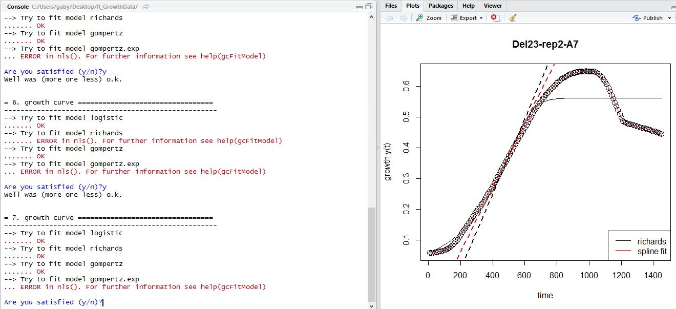

Reading summary table results:

The table summary file produced by Grofit will give you all the parameter values (mu=GrowthRates, lambda=LagPhaseTime and A=MaxAbsorbance) generated from the best model fits. Grofit uses 4 possible models; see documentation for more information.

References

1. https://www.jstatsoft.org/article/view/v033i07
2. https://cran.r-project.org/web/packages/grofit/index.html